Gerhard Buck-Sorlin, Institut Agro Rennes-Angers

Installing the platform GroIMP on your computer is actually quite straightforward if you carefully follow the instructions below. GroIMP runs on Java, so first of all, make sure you have a recent version of Java installed. To check if you have Java installed on your machine you open the command prompt window (type cmd in the search window), then type “java -version”, followed by Enter:

I have version 22 on my computer, which is one of the latest versions. If you don’t see this message or you know you don’t have Java, make sure to install Java version 22 before proceeding to the next step (you can find it here: https://jdk.java.net/22/)

Java 22 works fine with the latest version of GroIMP (2.1.5), which you will find here: https://gitlab.com/grogra/groimp/-/releases

On the Gitlab site, click on the link to the file GroIMP-2.1.5-win64.exe

if you have Windows on your machine like I have (else for Mac or Linux operating systems use one of the other files), to download the executable file. The following steps describe the procedure on Windows. For questions on how to install GroIMP on other operating systems, please do not hesitate to join the GroIMP group on Slack (groimp.slack.com) or the FSPM forum

Locate the downloaded file, double click on it (make sure you have administrator rights on your machine for installation), and follow the instructions one by one:

Normally, click on ‘I Agree’, then on ‘Next’. Choose the destination folder, then the maximum heap size for Java. This allocates a certain amount of RAM (random access memory) to the Java Virtual Machine on which GroIMP is running. By default, 1500 MB are allocated, but you can allocate up to 50 per cent of the RAM available on your machine to Java, without any problem (so on a machine with 10 GB RAM you can enter 5000):

After this you click on ‘Install’ and wait for the installation to finish (this can take more than ten minutes).

After the installation, a folder “GroIMP-2.1.5” should be available under something like this address: “C:\Program Files\”.

GroIMP will now be available either on your desktop or in the list of programmes:

Opening GroIMP should give a splash screen like this:

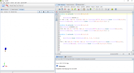
Then the platform should open, but you won’t see much yet, just an empty window with a menu on top. The first thing we want to do is to open an existing model called Alga.gsz: In the menu, go to “File” –> “Open”, then choose “Alga.gsz”¹⁾. (see also Appendix 1)

You should then see the following screen:

Note that on your machine, the naming of the menu items might vary, due to the language settings of your Java version (in this tutorial, the menu items will appear in English).
GroIMP is a multi-windows platform, i.e. it consists in fact of a (large) number of windows, which can be piled upon each other (like the sheets in an Excel file), “glued” side by side, or be viewed separately (this is handy if your computer is connected to more than one computer screen). To change the size of an integrated window you can simply click and drag on one of the grey hatched lines separating two windows. To change the position of a window you can click on the tab, hold and drag the whole window to its new position. You will see on your left a window called “View”, which contains the visual output of a model (currently a blue cylinder on its side, with a label “A” below it) and on your right a window called “jEdit – Alga.rgg”, in which you see the code of the model (you can scroll down the code using the slider on the right of the window). Another important window is located on the top left of your screen: on it you will find four buttons:

The buttons “run” and “Run run” serve to run the model. Unless you are told so, do not use the “Run run” button for the time being, as in some models (like the current one!) it will carry out the rules indefinitely, which might crash the programme and necessitate a restart. In fact, you will have to quickly press the “stop” button to prevent this. When you have run the model for a few steps you might want to go back to the beginning. Use the “Reset” button for this. If you just want to go back by one step (“undo the last step”), then use the button to the left of Reset: The disk button beside it will serve to save the whole project file:
If you modify the code you can save it afterwards using the save button of the jEdit window:

Apart from saving the code, this button will have an effect similar to the reset button, by letting you go back to the starting point of the model.

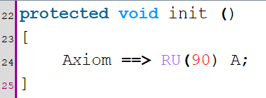
Let’s have a closer look at the code (in the jEdit window). By the way, jEdit is an external code editor, which will highlight reserved words and other parts of the code, thereby making it more readable. Scrolling down to line 22 (the line numbers can be found on the left of the jEdit screen), you will see the following code:

The text in line 24 is a rule, with a left-hand-side and a right-hand-side. The keyword ‘Axiom’ refers to the start word of the L-system, and ‘==>’ is an operator that essentially means “replace the left-hand side with the right-hand side”. Delete the semicolon and save the code. What happens is that the code will not be compiled. Instead, you will find in the Message window on the bottom of the jEdit window the following error message:

Note that the rule has to end with a semicolon (;) : omitting this will result in the error message above. This error message is rather helpful as it points exactly to the place where something has gone wrong and indicates what has to be modified: concretely, here it says: I actually expected a semicolon instead of the square bracket, so to rectify the code insert a semicolon before the square bracket, ] ). (You will have to get used to the fact that error messages are often pointing to a place in the code just above/before, so the error might be in the line above, as is the case here). By the way, another sign that your code is presently not functional is that the buttons (reset – stop – run – Run run) will disappear in case of an error in the code:

Reinsert the semicolon at the end of line 24 and save the code.

Let’s have a closer look at the code surrounding the Axiom rule:

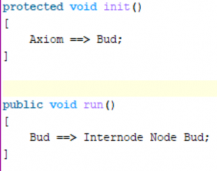
protected void init ()

init () is what is called a method in the Java language. Whenever you see a name followed by a pair of simple brackets, (), you can be almost certain that you are dealing with a method. A method is a little programme within the programme, a procedure that does stuff. The method init() carries out the Axiom rule. It is preceded by two key words, protected and void. protected refers to the type or visibility of the method. Here it means that the method is not visible to, or directly invokable by, the user. void refers to the type of output of the method. Java methods can be written such that they output a result of a certain type as we will see later. Our init() method just carries out a rule, but returns nothing otherwise, therefore its type is void, which means something like “empty”. Note that we also have a pair of square brackets surrounding the Axiom rule, [ and ] in lines 23 and 25, these are necessary to mark the beginning and end of the method code.
Next, have a look at the following code:

It is another method, named run(), void like the init() method (i.e. just doing stuff but returning nothing), but its type is public. This means the user can actually directly carry out this method by pressing the run (or Run run) button on the upper left panel that we have looked at before. The run() method contains three rules that we already dealt with in the lecture. They describe the development of the filamentous cyanobacterium (formerly known as blue-green alga) species Anabaena catenula, which was used by Aristid Lindenmayer to create the first L-system.
Press the run button (not Run run!) a few times and observe the output in the View window. The coloured cylinders representing the three different cell types are also labelled with a letter below, to help you understand what is going on. As we have explained in the lecture, each time you press run you rewrite the string by applying one, two, or all rules to the symbols in the string. At the start of the model, the string just consists of two things, RU(90) and A. RU(90) is a turtle command, which turns the head of the turtle down so that it is horizontal. It does this by performing a 90 degree turn around the back (UP or U) of the turtle. When the user presses the run button once, the program looks at the three rules in the method run() and checks if it can find a symbol in the current string, that occurs on the left-hand-side of one (or more…) of the rules.

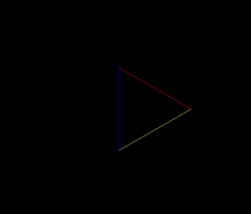
Open Ex01.gsz (Appendix 2): This model shows in the View window a triangle, and in the code just one method, init(), which as we have seen before, contains the Axiom rule. The start word (Axiom) is replaced by a series of six turtle commands, three times F(10) (drawing a line of length 10), and after each F a rotation command RU(120), which carries out a rotation around the UP vector of the turtle (we had this example in the lecture).
In the code you notice some text (the instructions for you) that is written in red, between /* and */. This is a way to comment the code. Everything between /* and */ will be ignored by the compiler of GroIMP, even if it is a longer text across numerous lines. If your comment fits onto one line, you can use // (as you can see in line 11 of the code).

Task: At the moment the tip of the triangle is pointing to the right. How can you turn the triangle such that it is resting on one of its sides?

Open Ex02.gsz (Appendix 3). This model looks similar to the previous one, only that the triangle in the View window is slightly turned (how? Check the code in the Axiom rule). The method init() is almost identical. However, now we have a public method called application(), and because it is public, two new buttons have appeared in the window on the top left: . Like before, do not press the button “Run application” as it will crash the model inevitably! Let’s have a look at the content of the method application. It contains a single rule involving F:

F(x) on the left-hand side (LHS) is replaced by 4 times F(x/3) on the right-hand-side (RHS) of the rule. This is actually already a parametric L-system, because the F has a parameter x (its length, which is equal to 10 in the beginning, see Axiom rule). And because we are using x on the left- and right-hand side of the rule, we can make sure that the length of the F at the left-hand side of the rule is taken over to the right-hand side. In other words F(10) on the LHS becomes F(3.33333) on the RHS. Other than that we have three rotation command, twice RU(-60) and once RU(120). Together with the replacement of one F by four smaller Fs, this gives the fractal that is known as the von Koch curve. Click a few times on application (not “Run application”) to observe the transformation of the triangle into a snowflake (we had this model in the lecture).
By the way, we learned in the lecture that the stuff we see in the View window is actually only an interpretation of the string by the turtle. Where is the string? Click on the window tab “Textual Overview” to see the string. In the beginning it looks like this:

Note that the string is preceded by the words “Node” and “RGGRoot” and that the string is bordered by two square brackets [] like the rules. All strings in GroIMP are actually graphs and they all have to start by these two initial nodes. You also see that at the start there are 8 nodes (the six turtle commands from the Axiom rule, plus the two initial nodes). After carrying out application once, this increases to 26 (the initial two nodes, plus the initial three RU commands, plus 3 times 7 new turtle commands that originate from replacing F). This increases to 98 in the next step, then 386, 1538, 6145, 24577, 98305, 393217… we stop here as the string rapidly becomes too long to be counted.

Open Ex02c.gsz (Appendix 4). This model will in fact simulate a simplified real tree, in which we have alternating branching, which get ever shorter and thinner the higher up we go. First of all, because we now need something like a “bud”, we had to declare for this model a new letter of the alphabet, A. This was done by declaring A as a module (line 6):

module A;

Note that the line has to end with a semicolon (;) and that the word module is written in small letters as it is a reserved keyword (so we can’t write Module or MODULE). A can now be used in the following. Like in the previous example we have put in the Axiom rule an F0 (stem) preceded by turtle commands for length, diameter, and colour, but now we have also inserted A (the bud) at the end. This becomes important in the method application, because here A is used on the LHS, it will be replaced by a rather complicated looking RHS: first of all, the turtle commands LMul(0.9) and DMul(0.9) are used to diminish the length and the diameter of the following F0 by 10 %. What follows are four more turtle commands, RU(90) F0 RU(-20) F0, i.e. rotations around the UP vector of the turtle by plus 90 degrees and then back -20 degrees, and twice F0. However, these commands are surrounded by a pair of square brackets. From the lecture you might remember that this designates a branch: when the turtle encounters the opening square bracket, [, it stores its current position and orientation into a stack (a kind of memory), and then moves on interpreting the commands after the opening square bracket, until it attains a closing square bracket: this is the command for the turtle to look into the stack and recover the last state, i.e. its exact position and orientation at the time it encountered the [. In this way, arbitrarily many pairs of square brackets, even stacked ones, can be interpreted by the turtle, but each [ must be matched by a ], otherwise this will produce a compilation error.
Click on the application button a few times: the initial stem produces further, ever thinner and shorter, stems, plus branches consisting of slightly bent-up stems (the effect of the command RU(-20)):

How do we get the alternation of branches (left and right following upon each other)?

Open Ex02d.gsz (Appendix 5). By now you should be a bit familiar with the code. In this example, we have declared two modules, A and B, because we wanted to model a bud A that can produce stems and branch, and a bud B that cannot (it will simply produce further stems). Inspect the model. Note that we cannot (yet) see A and B, we just see their respective effects when we press the run button a few times.
Change the global diameter, colour and length of the stems! Make the branches alternate!

Open Ex05.gsz (Appendix 6). When you run it by pressing run several times you will note that it produces a tree with alternating branches. Find out yourself how this has been done! Hint: it has something to do with the second parameter of the module B, ang, which is in fact determining the branching angle. In the rule in line 28, you can see that this second parameter is referred to as w.

Open Ex06.gsz (Appendix 7). This brings back a model we had a bit earlier, the model of Schoute. However, when you run it now, it will no longer be flat but completely 3D. Have a look at the rule in the run() method:

B(x) is the Bud, and I(x) the internode. We have again rotations around the UP axis, RU(30) and RU(-30), but these are followed by rotations around the HEAD axis of the turtle, RH(90). It is these rotations which turn the structure into a true 3D architecture.
What happens if you replace 90 degrees by 180 degrees?

Open Ex07.gsz (Appendix 8): This model works again with the snowflake (Koch) curve, with a triangle as starting structure:

Note, however, that the sides of the triangle are now colored, red, blue and yellow. Have a look at the Axiom rule to see why:

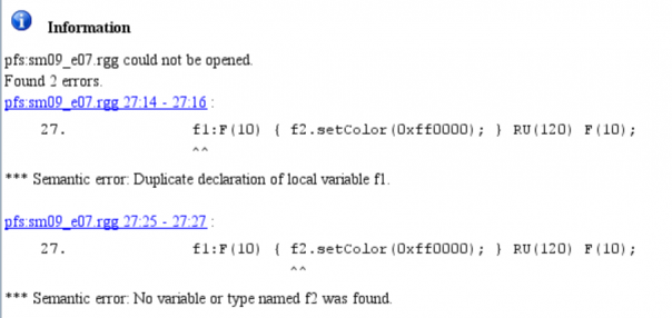
What has happened here? Instead of simply using F (with an argument in brackets) we have used f1:F(10) and f2:F(10). This is called “assigning a name to an object”. In other words, using a unique name (f1 and f2), we have identified the first two F(10) (note that we have not done this with the last F(10)). The way to do it is to use a unique short name followed by a colon (:) and the designation of a (previously defined) module or a known turtle command (which is an object, too). Change the first f2:F(10) to f1:F(10) and save the code. When you do this, the buttons on the top left of the screen will disappear, and a message appear in the window “Messages”:

You have declared the local variable f1 twice, which is not allowed as it should be unique like we said before, and also (2^nd error message), the variable f2 that appears in the same line is now unknown, as it has not been declared before. Change f1 back to f2 and recompile. Now let’s have a look at the code within the curly braces, {…} right behind the F10: This is so-called imperative code, as often used in programming languages like Java (in fact, the language you are using here, called XL, is a mixture of L-systems and Java). The expression {f1.setColor(0x0000ff);} sets the color of the object F named f1 to the value “0x0000ff”. In fact, this strange expression 0x0000ff is a hexadecimal number (you already know the decimal system in which we count from 1 to 10, or rather from 0 to 9, or the binary system, which only knows 0 and 1. In the hexadecimal system we count from 0 to 15, so we say the “base” is 16 and the digits are expressed as the numbers 0 to 9 followed by the letters A to F). The first two letters/numbers refer to red, the next two refer to green, and the last two refer to blue. The color values are defined in values between 00 and ff. ff is 256 in decimal but as you see we can write it shorter in hexadecimal: ff = 16*16 = 256. We can thus have 256 different reds, blues and greens, and all combined (256³) this gives roughly 16 million colors. setColor is a method of the turtle command F (if you are interested you can look up the definition of all classes of XL, including the turtle commands in the API documentation:)

This method accepts the hexadecimal color value 0x0000ff and interprets is as pure blue. So what then, is the color 0xff0000? You see that the last F is yellow? Why? How can you change its color from yellow to fuchsia?

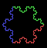
Press the derivation button once: the snowflake appears but everything is yellow now! Have a look at the rule in the method derivation to see why: in fact, when this rule is carried out, any F(x) (where x represents the length of the line, initially 10) is replaced by four new F, but in this rule no colours are specified. The specific objects f1 and f2 and their colors are only defined in the Axiom rule, not afterwards in the derivation rule. In this rule, they are thus replaced by new F whose color is undefined and thus yellow. How do you have to rewrite the code to keep the colors (see following picture)?

(Hint: use the fact that the turtle command F has three parameters: length, diameter, and color, where the latter can be indicated as a simple number between 0 and 15).

Open Ex08.gsz (Appendix 9). Again, we are working with the Koch snowflake curve. You might have noticed that writing the right-hand-side of the derivation rule is quite tedious and error-prone, especially the rotations and their arguments:

F(x/3) RU(-60) F(x/3) RU(120) F(x/3) RU(-60) F(x/3)

Suppose we want to change the angle of the RU rotation, from 60 and -60 to 55 and -55. We could do this manually by changing all the arguments one by one (note that we replaced 120 by 2*55=110):
F(x/3) RU(-55) F(x/3) RU(110) F(x/3) RU(-55) F(x/3)

Or we define two new modules like this:
module Rplus extends RU(60);

module Rminus extends RU(-60);

And in the rule we replace RU(-60) with Rminus and RU(120) with Rplus Rplus:

F(x) =⇒ F(x/3) Rminus F(x/3) Rplus Rplus F(x/3) Rminus F(x/3);

This way coding becomes much easier because we only need to change the value once, namely in the module definition. In the module definitions, substitute 60 by 50, and -60 by -55, and observe the effect! (Certain parameter combinations will remind of the tertiary folding of proteins). Abstain from pressing the “Run derivation” button!

Open Ex09.gsz (Appendix 10). In the example Ex03.gsz you already came across this tree model, it described the architecture of a forking tree, i.e. where at the tip of each annual shoot we find no terminal bud but two lateral buds opposite each other and inclined at a divergence angle of 30 degrees. This yielded a very regular architecture, in fact completely deterministic and completely flat. This is not what we see in nature. In the example Ex06 we had already seen how we could make the tree crown 3D by introducing the 90° turn around the head of the turtle (RH(90)), this leading to a decussate branching and a distribution of branches in 3D space. In this example we are going to introduce leaves. First of all, we have to define a module for this:

module Leaf(float len, float width) extends Parallelogram(len, width)
 
{{setShader(GREEN);}};

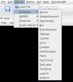
The leaf is defined as an extension of a Parallelogram object. You can have a look at how such an object looks like, by inserting it into the scene. For this, use the menu item “Objects” 🡪 “Primitives” 🡪 “Parallelogram”:

The Leaf module is defined with two parameters, len and width, both of type float (floating point number), which will be used to draw a parallelogram of length len and width width. Finally, the definition invokes the method setShader of Parallelogram to paint the leaves green. Note that for this you need to write {{ in the beginning, and }} at the end.

The leaf petiole is defined as an extension of F:

module Petiole(float len) extends F(len, 0.01);

The length len of the petiole is used by F, whereas the diameter is fixed (0.01), and the color of the petiole is not defined (it will thus be the default, yellow).

Have a look at the rule in the run method: You will find that instead of using a single number, some turtle commands will use an expression like this: random(20,45). random is in fact a library function that returns a uniformly distributed pseudorandom number between a minimum and a maximum number (the two arguments). We have used it here extensively to let the angles and the shoot lengths vary. Try out different maxima and minima and observe the effect. You can replace the uniform distribution with a normal distribution by using normal(mean, variance), where the first argument determines the mean value and the second the variance (if you have measured only the standard deviation you would have to take the root of this value).

Open Ex10.gsz (Appendix 11). In this example we will learn how to insert textures and images into a scene. You can start by going to the window called “Shaders” and double click on the object called “Leaf2”:

Make sure you do this quickly otherwise you might see this happen:

In fact “slowly double clicking” on the name opens the editor to rename the shader, which we don’t want right now (but it’s good to know anyway).
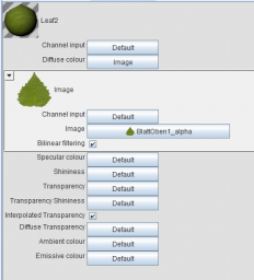
When you have double clicked correctly you should see the Attribute Editor appear with the Shader properties open:

You will see that the shader for the leaf object is already defined as an image (with a long, German sounding name…). Click on that name and choose another image, “GalaLeaf1”:

Notice that when you have already produced a structure, the effect is immediate, i.e. the leaf textures will change to the new image instantly. Otherwise you will see it when you develop the structure by pressing run a few times. By the way, you can also create your own (leaf) textures. Here’s how it’s done: Instead of clicking on “Project Images” you click on “from File”, then select an image file (preferably in png format) that you have prepared with, e.g. a tool like GIMP or ImageJ (for now you can simply download an image of a leaf from the internet and use that).

Open Ex11.gsz (Appendix 12). Here you will learn how to declare and use constants, and how to make the application of a rule depend on a condition. First of all, what do you need a constant for? Well, when you use a model parameter in your code whose value is not going to change during the simulation, you can use a constant. You could, of course, also simply use the value as a number but this could be tedious if the parameter is used a lot in the model. Here’s how a constant is declared:

We declared two constants, APICAL_REDUCTION-FACTOR, and STRENGTH_LIMIT. Notice that we use all capital letters to designate the names. This is a convention for constants to distinguish them from variables (which can, and will, change their value during the simulation), the latter being designated in lowercase letters. The reserved word “const” is followed by the type of the constant (here “float”), then the name and the value given. This is practical because now when you want to change the value of the constant you only need to do this once, where the constant is defined, because in the code you are going to use the NAME. Next, have a look at the rule within the method called grow:

You see that the Bud, which has a parameter strength, is “named” using b:Bud, so that we can use a condition: The condition is the expression immediately following the symbol on the left-hand-side, separated by a comma: (b[strength] > STRENGTH_LIMIT). We are effectively asking whether the variable “strength” of the Bud b is larger than the given value of the constant STRENGTH_LIMIT. Only if this is the case, the rule will be carried out, otherwise the Bud will stay “dormant”. So, to sum up, a condition is a logical (or Boolean) expression that will give “true” or “false”, and which can control the execution of a rule. We can use “>” and “<” but also “==” or “!=” when we are interested in checking whether a variable is identical or not identical with a given value. Notice that the constant APICAL_REDUCTION-FACTOR is used to reduce the strength x of the newly inserted terminal Bud, whereas the strength of the lateral buds is systematically reduced by multiplying with a factor 0.7.

Task: Change the values for the constants which are defined at the beginning and compare the resulting behaviour!

Open Ex12.gsz (Appendix 13). In this example you will learn how to keep the branching order as a parameter and how to get access to its value in a condition. In fact, you will learn a bit more about the branching order later. First of all, we will declare a constant:

This constant is of type integer and restricts the maximum branching order to 2. Next, since it is the Bud which is going to carry the information about the branching order, we need to give the Bud a new parameter, let’s call it order:

When the first Bud is initiated in the Axiom rule, we write

,

to designate a bud with order 0 and strength 5. In the actual production rule, several things are happening:

The order of the bud is referred to with the letter o, but like before we also use the “name” b for the Bud to be able to refer to its parameter order in the following condition,

(b[order] ⇐ MAX_ORDER_ALLOWED), where “⇐” means “is smaller than, or equal to”. Every new terminal bud inherits the order o of the mother bud, whereas in every new lateral bud the order o is increased by 1, o+1. This ensures that buds with order 3 will simply stop developing.

Open Ex13.gsz (Appendix 14). Here you will learn how to connect two conditions logically. In line 16 of the rgg file we have inserted a new constant:

STRENGTH_LIMIT is a constant parameter that we are going to use to define a certain lower limit of the strength variable of Bud. Have a look at the new condition in the production rule of the method grow:

(b[order] <= MAX_ORDER_ALLOWED && b[strength] > STRENGTH_LIMIT)

We see a new condition, b[strength] > STRENGTH_LIMIT, and it is connected to the old one by using “&&”. This “logical AND” means that both conditions need to be true before the rule can be applied. There are other possibilities: for instance, if we had used “||” instead (“logical OR”), it means that only one of the two conditions need to be true for the rule to be applied. This could be used in cases where several different circumstances lead to the same outcome.

Task: Change the values for the declared constants and compare the behaviour with both preceding examples!

Open Ex14.gsz (Appendix 15). We leave the tree model for a moment to look at a much simpler model, a stem without branches. This will help us to introduce the concept of how to modify properties of objects by actualization (or updating) rules. You have already learned how to put into place objects using production rules, thereby creating chains of objects with or without “side objects” (ramifications); we call the connections of these objects their topology. However, we do not yet have a means to control the development of the dimensions of the produced objects in time. In the definition of an object we can define its properties such as length, diameter and colour, and then we specify these variables with some (final) value that will not change afterwards. To model growth, these “internal” variables need to change (increment) in time, but we do not want the object to be replaced by a new object all the time, like we have done before. Instead we are going to use an actualization rule (in French you could call it “une règle de mise-à-jour). Let’s first have a look at the two modules: An Internode module is defined first:

This module has two parameters, age (because the Internode will age, i.e. become older with time), and f, both of type integer, i.e. they will typically be incremented by adding 1. Note that it extends F, whereby very small values for length and diameter are given (the initial size of the internode being small as we intend it to grow). The colouring of the Internode is very strange, but you will see that it will help us to distinguish the different internodes: we use “if“ and “else” and the condition “(f==0) to paint the internode either green or blue, depending on whether f is zero or not. The definition of the module for the Meristem is:

,

which gives a red sphere in appearance. Meristem has the same two parameters, age and f. In the Axiom rule, a Meristem is inserted, with age = 30 and f=0:

The public method run contains three rules. The first one replaces the Meristem with an Internode and a new Meristem, under the condition that its age is exactly 30.

This is done by identifying the Meristem by a name “m”, which is then used in the condition (“m[age]”) and to pass on the current value of f to the Internode (“m[f]”) and the new Meristem (“1-m[f]”). This is to make sure to have consecutive values of f that alternate between 0 and 1 (if you don’t believe me, try this out in an Excel sheet…). Look back at the definition of the Internode and you see now that this will lead to an alternation of blue and green internodes. Also note that the Internode and Meristem receive age = 0, their initial age.
The second rule is a so-called actualization rule:

The left-hand-side looks similar to the last rule, only that the condition m[age]<30 is required to be true for the rule to be carried out. However, instead of the familiar replacement operator =⇒ we now see ::> instead. This is called an actualisation operator. In fact, in such a rule, the symbol on the left-hand-side is not replaced by the string on the right-hand side, but on the right-hand-side we find a state variable of the symbol that is updated, in this case “m[age]++”, which is a shorthand notation for “take the current age of the Meristem named m and increment it by one” (we could also have written “m[age]+=1” or even longer: “m[age]=m[age]+1”). Indeed, we make the meristem older by one day at every step, as long as its age has not yet reached 30.

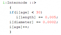
The third rule is again an actualization rule, but this time several variables of Internode are updated at once:

Length is incremented by 0.005 as long as the age of the internode has not reached 30 days, diameter is continuously incremented by 0.0002, without a condition, and internode age is incremented by one.
Task: Run the simulation by clicking on the “Run run” button. Change the length and diameter increment and the conditions, and rerun. For instance, how can you slow down meristem development or internode growth in length? How can you make short internodes, without slowing down meristem development?

Open Ex16.gsz (Appendix 16). Here you will learn the the use of a “for” loop on the right-hand side of a rule, for the automatic generation of several lateral branches at once. In the public method “lateralBranch”, for each F, its length x is taken as the turtle's step length ( L(x) ):

The rule continues as follows:

The keyword “for” starts a counting loop with 5 runs, where each run will generate a daughter branch. The variable i is an integer which is incremented by 1 in each run, giving 1 in the first run, then 2, 3, 4 and 5. The code to be repeated is put in brackets “(” and “)”. MRel is a turtle command that specifies the position of a branch at the mother shoot, and the argument is: (0.1*i+0.2). This will give the following five relative positions on the mother shoot: 0.3, 0.4, 0.5, 0.6, 0.7. The turtle command RU((-1**i)*30) lets the branching angle flip between -30 and 30 degrees (the expression (-1**i) has to be read as “minus one to the power of i”, and will give the series: -1, 1, -1, 1,… (again, don’t believe me but try this out on an Excel sheet).

Open Ex17.gsz (Appendix 17). You see here another example to work with imperative XL commands in order to update attributes of an object in actualization (update) rules. We first have defined a maximum value for the branching angle:

The following module definition is a bit special: Here you define your own rotation command derived from the turtle command RU: It inherits the attribute “angle” from its superclass RU. This attribute is taken over as parameter for the constructor by specifying it with “super.angle”.

(If you do not do this then GroIMP will issue a warning message but will nevertheless compile the code otherwise : try it out by writing “float angle” instead of “super.angle”!).

The Axiom rule is longer than usual, we actually specify the entire structure already here, a stem with two lateral branches, at two different insertion points and angles:

Note that we are using our own module Rotation instead of RU.
The public method changeAngle (for which you will have a button) contains an actualization rule for our module Rotation:

There are two conditions for this rule to be applied, and both concern the current argument of Rotation (identified here as “r”): In fact, the condition states that for the rule to be applied, the angle should be between MAXANGLE and -MAXANGLE. This might seem strange at first but in the if-else statement that follows you will see that it works, because if the angle is already negative it will be further decreased until it reaches -90 degrees, and if it is positive, it will be further increased until it reaches +90 degrees. Try out a value for MAXANGLE of 20, and see what happens! How can you slow down the angle increment on one side only?

In the remaining examples, it is your turn: You will slowly build a plant, from scratch as it were. I will help you with it, by providing the module definition, but it is up to you to write the code.

Open Unbranched.gsz (Appendix 18), the editor window on the right-hand side is still empty.

Write the following two rules in the editor window below the comment (“//simple stem, unbranched:”):

Axiom ==> Bud

Bud ==> Internode Node Bud

In order for this to work as a program, we have to write a bit more (by “wrapping” the rules with some method code):

run() is a public method. public: so that the user (you) can use it to run the model, and a method is a function that is carried out to run what is found inside, in this case the rule(s) are carried out. The name of the method doesn’t have to be run(), by the way: you can call it what you like, e.g. executer()

Now, change public to private, then save the code: The method disappears from the left-hand-side panel. Then change it back to public. The button appears again.

Click the run button a few times. Also, open the graph view (In the Menu go to “Panels, 2D, Graph”). Click on the objects and then inspect the Attribute Editor. In the graph view you see the actual data structure, the “graph”.

Move the object, zoom in and out, and turn it, using the corresponding tools.

Click , then , press stop QUICKLY. The potential danger of for certain quick models is that it fills up the memory and crashes or blocks your computer so that you have to restart GroIMP.

Open Leaves.gsz (Appendix 19)

Now, we are going to add leaves to the simple stem. Leaves are in some way “branches”, that is they are appendages inserted on the side of the stem and are not branching any further. Here is how you add leaves:

Insert the source code between Node and Bud: [ Leaf ]

then save and rerun by pressing a few times. Turn the plant using .

The leaves are normally not sticking to the branch, but instead they are inserted at a certain angle. To tell the program that it should put the leaf at such an angle, we use this rotation command: RL(70). You already know the turtle from the lecture: It has three axes around which rotations can take place. The RL-command will perform a rotation (R) around the left or L-Vector. You can also visualize the three vectors with the first three fingers of your (right or left) hand: thumb = UP, index = HEAD, middle = LEFT

Now save and rerun the model for a few steps. The rotation around the LEFT vector is also called “pitching down” (similar to a landing or sinking plane).

As you can see, the leaves are all pointing to one side, which is rather unnatural. Quite more often, leaves are arranged differently, for instance opposite each other. To create an alternation of leaves (i.e. one to the left, then one to the right, then again left, and so on), we could use the RL command again and tell it to pitch up or down alternately. However, this is not very elegant. A much easier way is to do a rotation around the head vector of the turtle by 180 degrees (by the way, this is called rolling, again in analogy to the movement of a plane) before a new bud is inserted. Let’s do this: Insert RH(180) before the Bud symbol.

Save and rerun. Finally, let’s insert another internode below the bud, because it seems the apical bud is sticking directly to the leaf. Insert Internode before RH(180).

Open Branches.gsz (Appendix 20).

Now we have a single stem with leaves, which endlessly produces new phytomers at the end. However, real plants produce branches, i.e. they produce new phytomers from lateral buds. So how can we teach the model to do this? First, let’s get rid of the leaves for reasons of simplicity, we will put them back in later. Comment the leaves out using /* */ (the code should look like this:
). In order to do branching we are going to reuse the Bud symbol in the branch: [ Bud ]. We have to add a rotation so that the new branch is growing out at an angle, for instance 50 degrees, RL(50):

Save and run for a few steps only. You see that the branched structure is completely flat, i.e. 2D. Let’s modify the RH command to make the plant branch to all sides, i.e. in 3 dimensions:

Insert RH(137.5) before the terminal Bud, then save and rerun:

137.5° is an angle very often encountered in nature: it is referred to as the “Golden Angle”. At this (so-called phyllotactic) angle, the least overlap and therefore self-shading of leaves within the same shoot occurs. This number goes back to the Fibonacci series: 1, 1, 2, 3, 5, 8, 13, 21, 34, 55, 89…

In this series, every new number is the sum of the last two numbers. When you divide two consecutive numbers (the smaller one by the bigger one = “ratio”), and multiply (1 – ratio) with 360, you get a value that approaches 137.5 degrees! (You can try this on an Excel sheet).

Put the leaves back in by removing the comments around the code: . As you see, the leaves are just another “branch” inserted at the node, but with a bigger angle, because the lateral bud is in the axil of a leaf and not the other way around. Run again, be careful not to use , just press the button repeatedly.

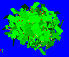
You get a real ball of leaves, with just one rule! Why do we get this? Because the Bud rule is unrestricted, it can always be applied, i.e. it has no condition attached to it.

Open BranchesRestr.gsz (Appendix 21).

However, what we really see in nature is, of course, a constrained growth of an organism, both in number of organs and in the growth of a single organ. We furthermore observe that the number of branching orders, e.g. in trees, is quite small, usually less than three or four.

Therefore, the way to restrict for instance branching order is to give the bud a parameter: Have a look at the new definition of the module bud:


Bud has now a parameter called order, and it is of type integer (int), which means it can be incremented by adding one each time we create a new branch. Orders are usually counted starting from 0 or 1. Let’s start with 1. When a module is used for the first time, we initiate the parameter by writing its value in brackets just behind the name of the module: As the bud should start with order 1 we write Bud(1) in the Axiom:

In the bud rule, we refer to the current value of order with the letter o: Bud(o). The compiler of GroIMP recognizes a parameter of a module from its position when it has more than one parameter (here, order is the only parameter of Bud, and therefore there is only one position). In the beginning this value is 1 (see the Axiom), in other words, when the production rule is applied for the first time, the value of o is one. On the right-hand side, we want to leave the order of the terminal bud as it is, so we also write Bud(o): the value of o (=1) is passed on to the new terminal bud. However, in the new lateral buds, order is incremented by one: Bud(o+1). What is missing now, is a condition: We want branching to stop when order 3 is reached, so we have to write

,(o⇐3) on the left-hand side, after Bud(o). The rule is thus only applied when the condition in parentheses is returning TRUE. More explicitly this rule now says: “If current order o of Bud is smaller or equal to 3, then replace Bud with right-hand-side, thereby creating two internodes, one leaf, a new terminal bud with the same order and one bud with order incremented by one. Else if order is larger than 3, do not carry out the rule (the bud will effectively stay dormant but will not die)”.

In the end the code of the method run should look like this:

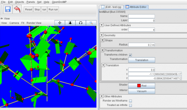
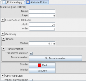
Save and rerun using only the button. Click on the terminal buds in the view window to see the parameter order. Then click on one of the lateral buds, its order has indeed increased to 4. And, as predicted, all the lateral buds with order 4 stop growing out.

However, if you manually lower the order of a selected bud and then press run again you will see that this bud will start to develop once more because the condition becomes TRUE. Try it out!

Open Phyllochr.gsz (Appendix 22).

Currently the shoots that grow do so at a high speed. This is because at every step, a new phytomer is produced at the tip of the shoot. If we want to change the speed at which new phytomers are formed, we have to introduce a parameter that puts the bud in a “dormant” state for a certain number of steps before the next phytomer is formed. The time between the appearance of two phytomers or more obviously leaves, is referred to as the phyllochron. It is convenient to define the phyllochron as a constant:

const int PHYLLO = 50;

The new constant is of type integer, has got the name PHYLLO (remember the convention to write constant is capital letters) and the value 50. (You can write this in Line 25, before the init method). In order to be able to use the phyllochron to determine the moment of bud outgrowth, we have to add a new parameter to the module Bud:

Note that the parameter phyllo is the first parameter, while order is now the second parameter (this is important as the compiler recognizes parameters in modules by their position).

We initiate the parameter (i.e. give it a concrete value) the first time the module is declared, in the Axiom rule:

Note that we didn’t write a number but instead used the name of the constant PHYLLO, then the program knows that it has to insert the number 50 every time the name PHYLLO is used. Later, we can change this number more easily in the declaration of the constant PHYLLO. What should be done with this number by the model? The idea is that it should count down from 50 (the current value of PHYLLO) to zero, before producing the next phytomer. The module Bud refers to this parameter under a name, so let’s call it p. p can have values between PHYLLO and 0. If p is larger than zero, it should be reduced by 1. Whenever a new Bud is inserted at the tip of the shoot or at the sides, the parameter should be re-set to the value of PHYLLO, because this new Bud has to wait and “count down” its own value of p from PHYLLO to zero before it can grow out itself. We now have two cases: p>0: wait and p==0: grow. Thus, we need to write a new rule, a kind of “dormancy” rule:

Bud(p,o), (p>0) =⇒ Bud(p-1,o);

Moreover, we have to modify the existing rule:

The condition is enlarged (we use “&&” to concatenate two conditions, this means “AND”, so both conditions need to be true): (p==0 && o⇐2)

(note that we set the maximum order to 2 now). On the right-hand-side, the two (new) buds are each initiated with PHYLLO:

Bud(PHYLLO, o+1) resp. Bud(PHYLLO, o)

After all these changes, your run-method should look like this:

Save and rerun now. Change the value of PHYLLO (for instance to 100 or 25) and observe the effect on the speed of development! Check out the values of p by clicking on different buds, you can also manually change these values in the Attribute editor:

Open Flowering.gsz (Appendix 23).

Now, plants don’t stay vegetative forever. In fact, what you observe in many plants is that an apical meristem, after having formed a certain number of phytomers, will decide to form a terminal flower and thereby use itself up, i.e. there will be no further formation of phytomers. Let’s tell the bud to produce a flower once it has formed a given number of phytomers. In order to do so, we have to introduce a new parameter to the bud, r (for rank), which is counted up to 10, and if r == 10, it produces a flower. First, we change the axiom rule (r is initially 1):

Then, we need a new rule for the flower, which is inserted after the two rules in the run method:

Bud(r,p,o), (r==10) =⇒ Internode Internode Flower;

Finally, we need to modify the first and the second rule of the method run() by adding a new condition: As long as r is smaller than 10, a phytomer is produced:

Bud(r,p,o), (r<10 && p==0 && o⇐2)

r is incremented by 1 in the terminal bud, otherwise it stays the same value, thus

Bud(r+1,PHYLLO,o+1) for the terminal bud, and Bud(r+1,PHYLLO,o+1) for the lateral bud.

Now finally, let’s insert a turtle command which improves realism by bending the shoots slightly upwards:

RV(-0.1)

Insert this command before the first two Internode modules.

Your run method should now look like this:

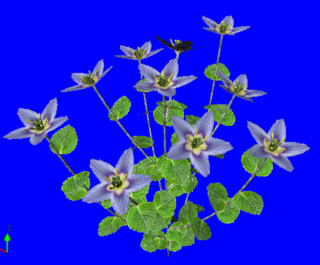
You now get a flowering plant, it looks ok, but not really nice.

Insert the word Joli before each module (without a space), JoliInternode, JoliNode, JoliLeaf, and JoliFlower. Save and run again, you should now get something like this:

Of course, Joli is not a magic word. Instead, we had to define all the modules we were going to use in the model beforehand.

Have a closer look at the module definitions.

I have done this for all the examples in order to make things easier for you to understand. These modules have to be defined as objects with certain known features, with or without geometric features. For instance, a bud can be defined as a red sphere with a color or texture, a leaf a green rectangle (or parallelogram) or instead with a texture mapped onto it, showing the picture of a photographed or scanned leaf.

Task: change the texture of the leaf using another image!

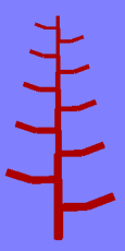
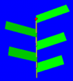
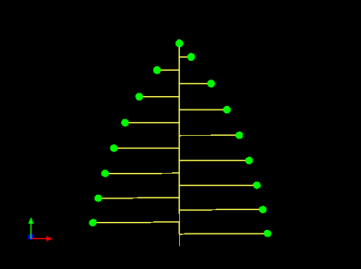
Now try it on your own: Here is a tree that I constructed using two lines of code and two modules, A and B. Write the code that will create the tree!

Hint: A is used for the stem, B for the branches.

module A extends Cylinder(0.2,0.2)
{
	{setShader(BLUE);}
} ==> [ RG  M(0.5) RU(-90) M(0.1) TextLabel("A").(setColor(new Color3f(0,0,0)),
setFilled(true), setFillColor(new Color3f(0.9,0.8,0.7))) ];
 
module B extends Cylinder(0.2,0.2)
{{setShader(GREEN);}}
==>[ RG M(0.5) RU(-90) M(0.1) TextLabel("B").(setColor(new Color3f(0,0,0)),
setFilled(true), setFillColor(new Color3f(0.9,0.8,0.7))) ];
 
module C extends Cylinder(0.2,0.2)
{
	{setShader(new RGBAShader(0.9, 0.5, 0.1));}
}
==> [ RG M(0.5) RU(-90) M(0.1) TextLabel("C").(setColor(new Color3f(0,0,0)),
	setFilled(true), setFillColor(new Color3f(0.9,0.8,0.7)))];
 
 
 
 
protected void init ()
[
	Axiom ==> RU(90) A;
]
 
public void run ()
[
	A ==> A B;
	B ==> A C;
	C ==> B;
]

/*
You learn at this example:
- how to create a simple model of a triangle as a static structure
- how to insert comments into the code
*/
 
protected void init()
[
   //    The start word is transformed into a triangle
   Axiom ==>  F(10) RU(120) F(10) 
   		RU(120) F(10) RU(120);
]

/*
You learn at this example:
- how to modify a simple model of a triangle to extend it to a Koch curve
- your first "proper" rule application
- the definition of a public method "application" (rule application)
*/
 
//---------------- Example Koch curve   -------------------------------------
// each line will be replaced by 4 lines with length = (original length / 3)
 
protected void init()
[
   Axiom ==> RU(50) F(10) RU(120) F(10) RU(120) F(10);
]
 
// public method for the interactive use in GroIMP (via button)
public void application()
// rules must be put in [] - brackets and must be finished with ;
[
   // each F() is replaced by 4 smaller F()
   // the length of the F at the left-hand side of the rule
   // is taken over to the right-hand side
   F(x) ==> F(x/3) RU(-60) F(x/3) RU(120) 
   		F(x/3) RU(-60) F(x/3);
]

//------ Example: alternating branches with successive shortening   -------
 
/* A is not a turtle command, thus it has to be declared as a "module"
   before it can be used in the L-system: */
 
module A;
 
protected void init()
   [
   Axiom ==> L(10) D(3) P(4) F0 A;
   ]
 
// public method for the interactive use in GroIMP (via button)
public void application()
   [
   A ==> LMul(0.9) DMul(0.9) [ RU(90) F0 RU(-20) F0 ]
   F0 RH(180) A;
   ]

module A;
module B;
 
protected void init()
   [ 
   Axiom ==> L(1) A; 
   ]
 
public void run()
   [ 
   	 A ==> F0 [ RU(45) B ] A;
     B ==> F0 B; 
   ]

/*
You learn at this example:
how to create a simple model of shoot growth with alternating
positioning of lateral branches.
*/
 
// definition of a terminal bud as extension of a sphere
module B(float len, float ang) extends Sphere(0.1)
{{setShader(GREEN);}}
 
// definition of a lateral bud as extension of a sphere
module LB(float len) extends Sphere(0.1)
{{setShader(RED);}}
 
// definition of an internode as extension of the module F
module I(float len) extends F(len);
 
// start method with the axiom (generates a bud)
protected void init()
[
   Axiom ==> B(1, 70);
]
 
public void run()
[
   B(x, w) ==> I(x) [ RU(w) LB(0.6*x) ] B(0.95*x, -w);
   LB(x) ==> I(x) LB(x);
 
]

/* You learn at this example:
- how to create a simple model of shoot growth with opposite
  branching (in 3d)
- how to use elements without drawing them (module B) */
 
// architectural tree model Schoute
// I for Internode extends the turtle command F
module I(float len) extends F(len);
 
// B stands for a bud and is not a visible object (is not drawn)
module B(float len);
 
protected void init()
[
   Axiom ==> B(5);
]
 
public void run()
[
   // rotation around the up axis (RU) and around the head axis (RH)
   B(x) ==> I(x) [ RU(30)  RH(90) B(0.9*x) ] 
                 [ RU(-30) RH(90) B(0.9*x) ];
]

/* You learn at this example:
- how to insert simple imperative XL code directly into a rule,
- how to assign objects (nodes of the graph) during their generation
  on the right-hand side of a rule by names and how to use them directly in XL code,
- that by replacement, all attributes get lost when the objects are replaced,
- that it is possible to transfer attributes from the left-hand side of a rule to its right-hand side, if you take care of this (e.g., the length of F is saved by the variable x) */
 
// the Koch curve again
protected void init()
// rule blocks must be enclosed in [] brackets
[
   // a coloured triangle as the start word
   // In braces { }, imperative XL code is specified: Here, the specification of the colour.
   // The Objects are directly named when they are generated (names f1, f2).
   Axiom ==> f1:F(10) {f1.setColor(0x0000ff);} RU(120) 
   			 f2:F(10) {f2.setColor(0xff0000);} RU(120) 
   			 F(10);
]
 
public void derivation()
[
   // replacement rule
   F(x) ==> F(x/3) RU(-60) F(x/3) RU(120) F(x/3) RU(-60) F(x/3);
]

/* You learn at this example:
how to define your own modules in order to simplify the code */
 
// Koch curve with module definitions for rotation operators
module Rplus  extends RU(59);	// rotation counterclockwise: try 55, 59
module Rmoins extends RU(-61);	// rotation clockwise
 
protected void init()
[
   Axiom ==> F(10) RU(120) F(10) RU(120) F(10);
]
 
public void derivation()
[
   // usage of the modules Rplus and Rminus for the rotation
   F(x) ==> F(x/3) Rmoins F(x/3) Rplus Rplus F(x/3) Rmoins F(x/3);
]

// Example for a simple tree architecture (model Schoute)
module Shoot(float len) extends F(len, 0.2);
module Bud(float strength) extends Sphere(0.2)
{{setShader(RED); setTransform(0,0,0.3);}};
 
// Definition of the leaf object as extension of a parallelogram:
module Leaf(float len, float width) extends Parallelogram(len, width)
{{setShader(GREEN);}};
 
module Petiole(float len) extends F(len, 0.05);
//----------------------------------------------------/
protected void init()
[ Axiom ==> Bud(5); ]
 
// rule system for Schoute architecture; notice the leaf objects (Leaf).
public void run()
[
   Bud(x) ==> Shoot(x)
      // for angle variations, random numbers are used
      [ RU(80) RH(90) Petiole(0.3*x) Leaf(x,x*0.33) ]              // Leaf 1
      [ RU(normal(30,10)) RH(random(70,110)) Bud(0.7*x) ]     // Branch 1
      [ RU(-90) RH(90) Petiole(0.3*x) Leaf(x,x*0.33) ]             // Leaf 2
      [ RU(random(-20, -45)) RH(random(70,110)) Bud(random(0.7,1.1)*x) ]; // Branch2
]

// Example for a simple tree architecture (model Schoute)
module Shoot(float len) extends F(len, 0.2);
module Bud(float strength) extends Sphere(0.2)
{{setShader(RED); setTransform(0,0,0.3);}};
 
// Definition of a global constant for the call of the texture:
const Shader leafMat = shader("feuille");
 
// Definition of the leaf object as extension of a parallelogram:
module Leaf(float len, float width) extends Parallelogram(len, width)
 
// the shader gets assigned a texture instead of a colour
{{setShader(leafMat);}};
 
module Petiole(float len) extends F(len, 0.01);
 
//----------------------------------------------------/
 
protected void init()
[ Axiom ==> Bud(5); ]
 
// rule system for Schoute architecture; notice the leaf objects (Leaf).
public void run()
[
   Bud(x) ==> Shoot(x)
      // for angle variations, random numbers are used
      [ RU(80) RH(90) Petiole(0.2*x) Leaf(4, 2) ]              // Leaf 1
      [ RU(random(20,45)) RH(random(70, 110)) Bud(0.9*x) ]     // Branch 1
      [ RU(-90) RH(90) Petiole(0.2*x) Leaf(4, 2) ]             // Leaf 2
      [ RU(random(-20, -45)) RH(random(70, 110)) Bud(0.9*x) ]; // Branch2
]

/* You learn at this example:
- how to use constants,
- how to make the application of a rule depend on a condition.
Change the values for the constants which are defined at the
beginning and compare the resulting behaviour. */
 
module Shoot(float len) extends F(len);
module Bud(float strength) extends Sphere(0.2)
{{setShader(RED); setTransform(0,0,0.3);}};
//----------------------------------------------------/
const float APICAL_REDUCTION_FACTOR = 0.9; //try 0.6 to 0.99
const float STRENGTH_LIMIT = 2.0; //try anything between 5 and 0.5
 
// Start block with the start word
protected void init()
[ Axiom ==> Bud(5); ]
 
// public rule block (appears as button in the menue)
public void grow()                                    
[
// condition is set (in parentheses (...) )
   b:Bud(x), (b[strength] > STRENGTH_LIMIT) ==> Shoot(x) 
       [ RU(50) Bud(0.7*x) ] [ RU(-50) Bud(0.7*x) ] 
       Bud(APICAL_REDUCTION_FACTOR * x);
]

/* You learn at this example:
how to keep the branching order as a parameter and how to get 
access to its value in a condition. */
 
module Shoot(float len) extends F(len);
module Bud(int order, float strength) extends Sphere(0.2)  // order as param.
   {{setShader(RED); setTransform(0,0,0.3);}};
 
const float APICAL_REDUCTION_FACTOR = 0.9;
const int MAX_ORDER_ALLOWED = 2;
//----------------------------------------------------/
// Start block with the start word
protected void init()
[ Axiom ==> Bud(0, 5); ]
 
// public rule block
public void grow()
[
   b:Bud(o, x), (b[order] <= MAX_ORDER_ALLOWED) ==> Shoot(x) 
      [ RU(50) Bud(o+1, 0.7*x) ] [ RU(-50) Bud(o+1, 0.7*x) ] 
      Bud(o, APICAL_REDUCTION_FACTOR * x);
]

/* You learn at this example:
how to connect two conditions logically. */
 
module Shoot(float len) extends F(len);
module Bud(int order, float strength) extends Sphere(0.2)
{{setShader(RED); setTransform(0,0,0.3);}};
 
const float APICAL_REDUCTION_FACTOR = 0.9;
const float MAX_ORDER_ALLOWED = 3;
const float STRENGTH_LIMIT = 1.5;
//----------------------------------------------------/
// Start block with the start word
protected void init()
[ Axiom ==> Bud(0, 5); ]
 
// public rule block (appears in the menue)
public void grow()
[
   // two conditions are specified
   Bud(o, x), (o <= MAX_ORDER_ALLOWED && x > STRENGTH_LIMIT) 
      ==> Shoot(x) [ RU(50) Bud(o+1, 0.7*x) ] 
          [ RU(-50) Bud(o+1, 0.7*x) ] Bud(o, APICAL_REDUCTION_FACTOR * x);
]

/* You learn how to modify properties of objects by actualization rules.
Objects and their connections control topology,
properties of objects (attributes) control geometry and colour. */
 
// a simple internode with a fixed, very small initial size
module Internode(int age, int f) extends F(0.02, 0.0005)
   {{if (f == 0) setShader(GREEN);
     else setShader(BLUE);}};
 
// a simple meristem
module Meristem(int age, int f) extends Sphere(0.002)
   {{setShader(RED);}};
 
// The initial structure consists of the meristem
protected void init()
[ Axiom ==> Meristem(30, 0); ]
public void run()
[
   // Two alternative rules for the meristem:
   // first rule for a new meristem: Creation of the internode
   m:Meristem, (m[age] == 30) ==> 
     Internode(0, m[f]) RH(140) RU(random(-30, 10)) Meristem(0, 1-m[f]);
   // The meristem ages by 1 day
   m:Meristem, (m[age] < 30) ::> m[age]++;
   // rule for the increase of the internodium
   i:Internode ::> 
      {
      if(i[age] < 100) 
         i[length] += 0.005;  // length growth: the first 30 days
      i[diameter] += 0.0002;  // Thickness growth always
      i[age]++;               // incrementation of the age
      }	
]

/* You learn at this example 
- the use of a "for" loop on the right-hand side of a rule
- the automatic generation of several lateral branches */
 
protected void init()
[ Axiom ==> F(10); ]
 
public void lateralBranch()
[
// for each F, its length x is taken as the turtle's step length ( L(x) )
   f:F(x) ==> f L(x)
 
// Counting loop (for) with 5 runs.
// Each run generates a daughter branch.
// The variable i is an integer which is incremented by 1
// in each run (1, 2, ..., 5).
for (int i=1; i<=5; i++) 
   (
// MRel(0.1*i+0.2) specifies the position at the mother shoot,
// starting at 20%, + 10% per run.
   [ MRel(0.1*i+0.2) RU((-1**i)*30) F(x*0.2) ]
// RU((-1**i)*30) lets the branching angle flip between
// -30 and 30 degrees.
   );
]

/* You learn at this example to work with imperative XL commands in order to update attributes of an object in actualization (update) rules. 
Watch the attributes of the objects in the attribute editor of GroIMP and the possibilities given there to change these attributes. 
It is also possible to have direct access to attributes of the superclass of the considered object there! */
// Definition of a CONSTANT: Constants are often denoted with CAPITALS.
 
const float MAXANGLE = 100.0;
 
// Definition of your own rotation command derived from RU:
// It inherits the attribute "angle" from its superclass RU.
// This attribute is taken over as parameter for the constructor
// by specifying it with "super.angle".
module Rotation(super.angle) extends RU(angle);
 
protected void init()
[
   // Creation of branching under use of the user-defined rotation module
   Axiom ==> L(10) F0
                   [ MRel(0.7) Rotation(-30) F(6) ]
                   [ MRel(0.5) Rotation(40)  F(6) ];
]
 
public void changeAngle()
[
   // use of an actualization rule ( ::> )
   r:Rotation, (r[angle] < MAXANGLE && r[angle] > -MAXANGLE) ::> 
      { // imperative code block
      if (r[angle] < 0)
         r[angle] -= 3;  /* shorthand for: r[angle] = r[angle] - 3; */
      else
         r[angle] += 3;  /* analogously */
      }
]	
 
/* An actualization rule is used to change attributes (properties) of objects (i.e., of nodes) by rule application. 
With this rule, no objects are replaced. The structure of the graph is not changed. 
Only the attributes of existing objects (nodes of the graph) can be updated. Rules of this type are marked by the ::> arrow.*/

module Bud extends Sphere(0.1)
{
	{setShader(RED);}
} 
 
module Node extends Sphere(0.07)
{
	{setShader(GREEN);}
}
 
module Internode extends F;
module Leaf extends Parallelogram(2,1)
{
	{setShader(GREEN);}
}
 
static boolean VISIBLE = true;
module Turtle extends Null
==> if(VISIBLE) (M(0.7) Sphere(0.4).(setShader(GRAY)) 
	F(1,0.1, 4) M(0.5) TextLabel("Turtle"));
 
//simple stem, unbranched:

module Bud extends Sphere(0.1)
{
	{setShader(RED);}
}
 
module Node extends Sphere(0.07)
{
	{setShader(GREEN);}
}
 
module Internode extends F;
 
module Leaf extends Parallelogram(2,1);
 
static boolean VISIBLE = false;
module Turtle extends Null
==> if(VISIBLE) (M(0.2) [ M(-0.26) RL(165)  Cone(0.1,0.04).(setShader(GRAY))] RH(45) 	s:SphereSegment(0.3) {s.setShader(GRAY);s.setTransform(0.002,0,0);} [M(0.1) RH(45) [ RU(20) RL(60) RH(90) F(0.2,0.05,4)] [ RU(20) RL(-60) RH(-90) F(0.2,0.05,4)] ] [M(-0.2) RH(45) [ RU(20) RL(60) RH(90) F(0.2,0.05,4)] [ RU(20) RL(-60) RH(-90) F(0.2,0.05,4)] ]M(0.2) SphereSegment(0.2).(setShader(RED)) M(0.5) TextLabel("Turtle"));
 
//Introducing leaves
protected void init ()
[
	Axiom ==>  Bud;
]
 
public void run ()
[
	Bud ==> Internode Node Bud ;
]

module Bud extends Sphere(0.1)
{
	{setShader(RED);}
}
 
module Node extends Sphere(0.07)
{
	{setShader(GREEN);}
}
 
module Leaf extends Parallelogram(2,1);
module Internode extends F;
 
 
//Introducing branching
protected void init ()
[
	Axiom ==> Bud;
]
 
public void run ()
[
	Bud ==> Internode Node [ RL(70) Leaf ] RH(180) Bud;
]

module Bud (int order) extends Sphere(0.0001)
{
	{setShader(RED); setRadius(0.2);}
}
 
module Node extends Sphere(0.07)
{
	{setShader(BLUE);}
}
 
module Leaf extends Parallelogram(2,1)
{
	{setShader(GREEN);}
}
 
module Internode extends F;
 
 
//Restricting the branching order
protected void init ()
[
	Axiom ==> Bud(1);
]
 
public void run ()
[
	Bud(o), (o<=3) ==> Internode Node [ RL(50) Bud(o+1) ] 
		[RL(70) Leaf] RH(180) Internode Bud(o); 
]

module Bud (int phyllo, int order) extends Sphere(0.1)
{
	{setShader(RED);}
}
 
module Node extends Sphere(0.07)
{
	{setShader(GREEN);}
}
 
module Leaf extends Parallelogram(2,1);
module Internode extends F;
 
//introducing a phyllochron
 
protected void init ()
[
	Axiom ==> Bud(1);
]
 
public void run ()
[
	Bud(o),(o<=3) ==> Internode Node 
		[ RL(50) Bud(o+1) ] [RL(70) Leaf] 
		RH(137)	Internode Bud(o);
]

module Bud(int rank, int phyllo, int order) extends Sphere(0.1)
{
	{setShader(nodemat);}
}
 
module Node extends Sphere(0.07)
{
	{setShader(GREEN);}
}
 
const ShaderRef leafmat = new ShaderRef("Lambert");
const ShaderRef petalmat = new ShaderRef("Lambert 2");
const ShaderRef internodemat = new ShaderRef("Lambert 3");
const ShaderRef nodemat = new ShaderRef("Lambert 4");
 
module Leaf extends Parallelogram(2,1).(setColor(0x82B417));
module JoliLeaf extends Parallelogram(2,2).(setShader(leafmat));
module JoliNode extends Sphere(0.07)
{{setShader(nodemat);}}
 
module Internode extends F(normal(1,0.2),0.1,7);
module JoliInternode extends Cylinder(normal(1,0.2),0.08).(setShader(internodemat));
 
module Flower ==> 
RU(180) Cone(0.3,0.3).(setShader(new RGBAShader(130/255, 180/255, 1/255))) M(-0.25) RL(90) 
[ for (int i=1; i<=5; i++) ([RU(i*360/5) RL(20) Parallelogram(2,1).(setColor(0xFF00FF))])]
	RU(45) 
	[ for (int j=1; j<=5; j++) ([RU(j*360/5) RL(40) F(0.3,0.1,14) RV(-0.3) F(0.3,0.1,14) RV(-0.3) F(0.3,0.1,14)]) 
	]
	RU(-45) 
	[ for (int k=1; k<=5; k++) ([RU(k*360/5) RL(70) Frustum(0.7,0.2,0.05).(setShader(new RGBAShader(141/255, 175/255, 5/255)))]) 
	];
 
module JoliFlower ==> 
RU(180) Cone(0.3,0.3).(setShader(internodemat)) M(-0.25) RL(90) 
[ for (int i=1; i<=5; i++) ([RU(i*360/5) RL(20) Parallelogram(2,1).(setShader(petalmat))])]
	RU(45) 
	[ for (int j=1; j<=5; j++) ([RU(j*360/5) RL(40) F(0.3,0.1,14) RV(-0.3) F(0.3,0.1,14) RV(-0.3) F(0.3,0.1,14)]) 
	]
	RU(-45) 
	[ for (int k=1; k<=5; k++) ([RU(k*360/5) RL(70) Frustum(0.7,0.2,0.05).(setColor(0x8DAF58))]) 
	];
 
//introducing flowering
const int PHYLLO = 25;
 
protected void init ()
[
	Axiom ==> Bud(PHYLLO, 1);
]
 
public void run ()
[
	Bud(p,o),(p>0) ==> Bud(p-1,o);
	Bud(p,o),(p==0 && o<=2) ==> RV(-0.1) Internode Node 
				[ RL(50) Bud(PHYLLO,o+1) ][RL(70) Leaf] 
				RH(137) RV(-0.1) Internode Bud(PHYLLO,o);
]